1X World Model Challenge
Introduction
World models equip agents (e.g., humanoid robots) with internal simulators of their environments. By “imagining” the consequences of their actions, agents can plan, anticipate outcomes, and improve decision-making without direct real-world interaction.
A central challenge in world modelling is the design of architectures that are both sufficiently expressive and computationally tractable. Early approaches have largely relied on recurrent networks or multilayer perceptrons. More recently, advances in generative modelling have driven a new wave of architectural choices.
A prominent line of work leverages autoregressive transformers over discrete latent spaces, while others explore diffusion- and flow-based approaches. At scale, these methods underpin powerful foundation models capable of producing realistic and accurate video predictions.
Overview of the 1X World Model Challenges
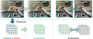
The 1X World Model Challenge (part of the Autonomous Grand Challenge 2025) evaluates predictive performance on two tracks: Sampling and Compression.
These challenges capture core problems when using world models in robotics.
The figure below illustrates the two challenges: Overview of the 1X World Model Challenges.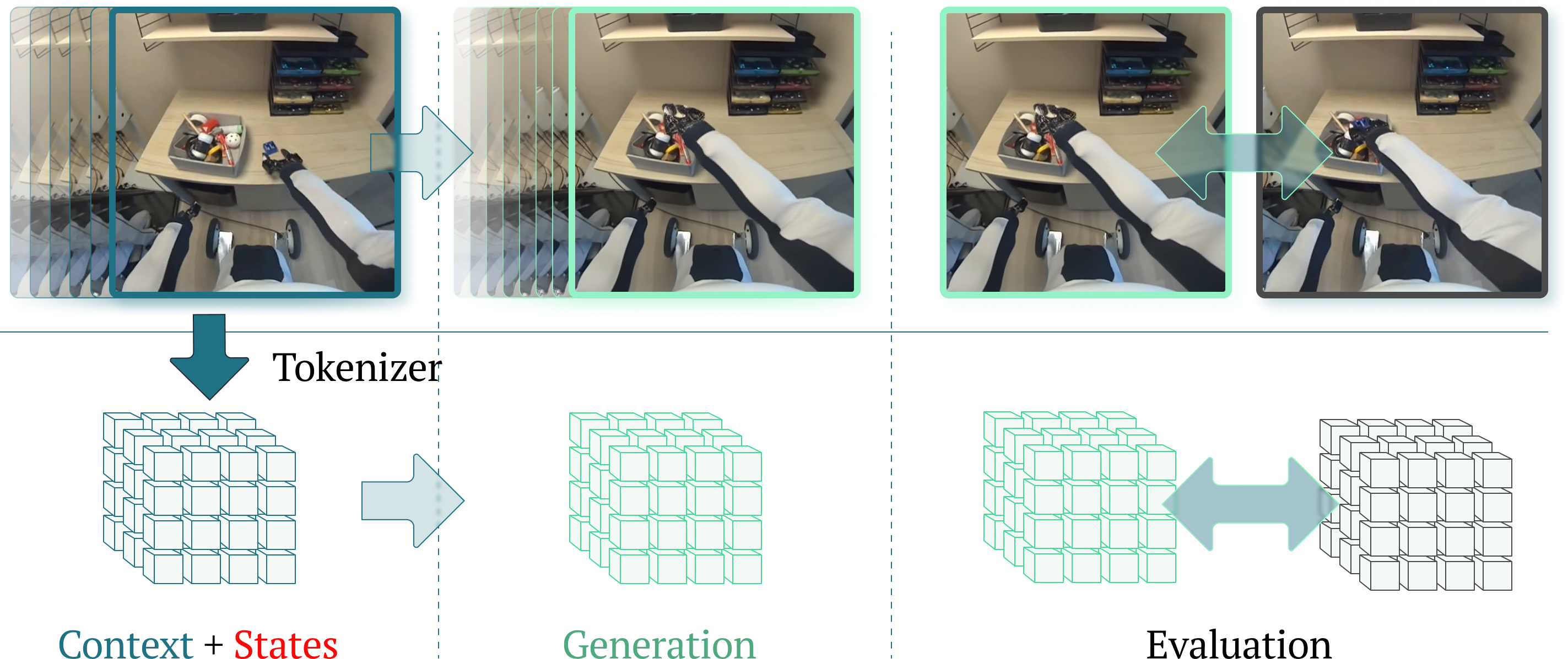
Compression Challenge
The Compression Challenge evaluates models in a discrete latent space. Each video sequence is first compressed into a grid of discrete tokens using the Cosmos $8 \times 8 \times 8$ tokeniser, producing a compact sequence that can be modelled with sequence architectures.
Problem Statement
Given a context of $H=3$ grids of $32 \times 32$ tokens and robot states for both past and future timesteps, the task is to predict the next $M=3$ grids of $32 \times 32$ tokens:
$$ \begin{align} \hat{\mathbf{z}}_{H:H+M-1} &\sim f_{\theta}(\mathbf{z}_{0:H-1}, \mathbf{s}_{0:63}) \end{align} $$where $\hat{\mathbf{z}}_{H:H+M-1}$ are the predicted token grids for the future frames. The tokenized training dataset $\mathcal{D}$ contains approximately $306{,}000$ samples. Each sample consists of:
- Tokenised video: $6$ consecutive token grids (3 past, 3 future), each of size $32 \times 32$, giving $6144$ tokens per sample and $\sim1.88$B tokens overall.
- Robot state: a sequence $\mathbf{s} \in \R^{64 \times 25}$ aligned with the corresponding raw video frames. A block of three $32 \times 32$ token grids corresponds to 17 RGB frames at $256 \times 256$ resolution, so predictions in token space remain aligned with the original video. Performance is evaluated using top-500 cross-entropy, which considers only the top-500 logits per token.
Model
For the compression challenge, we implemented a spatio-temporal transformer world model. Given three grids of past video tokens of shape $3 \times 32 \times 32$, as well as the robot state of shape $64 \times 25$ as context, the transformer predicts the future three grids of shape $3 \times 32 \times 32$. The ST-Transformer consists of $L$ layers of spatio-temporal blocks, each containing per time step spatial attention over the $H \times W$ tokens at time step $t$, followed by causal temporal attention of the same spatial coordinate across time, and then a feed-forward network. Each colour in the spatial and temporal attention represents a single self-attention map.
Spatio-temporal Transformer
Following Genie, our world model builds on the Vision Transformer (ViT). An overview is shown in the Figure below.
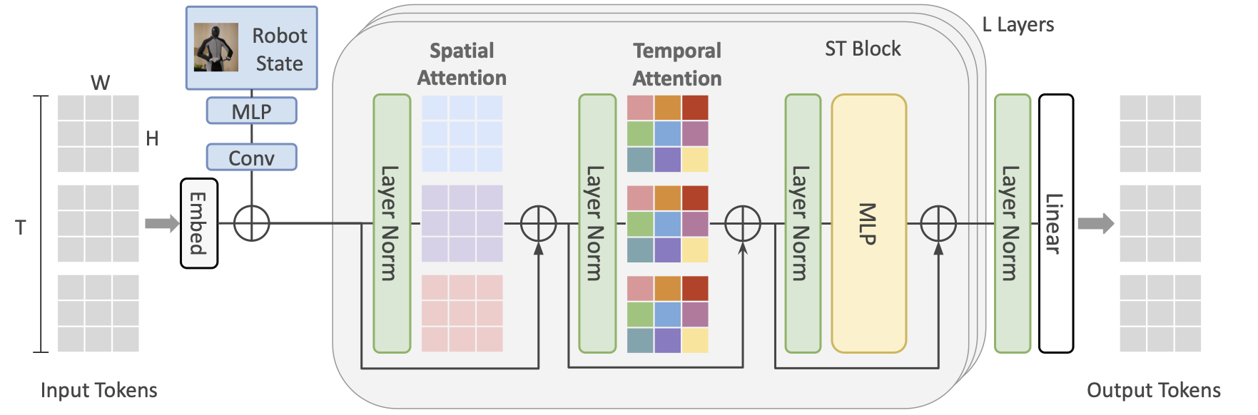
Illustration of our ST-Transformer architecture for the compression challenge.
To reduce the quadratic memory cost of standard Transformers, we use a spatio-temporal (ST) Transformer, which alternates spatial and temporal attention blocks followed by feed-forward layers. Spatial attention attends over 1 × 32 × 32 tokens per frame, while temporal attention (with a causal mask) attends across T × 1 × 1 tokens over time.
This design makes spatial attention—the main bottleneck—scale linearly with the number of frames, improving efficiency for video generation.
We apply pre-LayerNorm and QKNorm for stability. Positional information is added via learnable absolute embeddings for both spatial and temporal tokens.
Our transformer uses:
- 24 layers
- 8 heads
- Embedding dimension: 512
- Sequence length: T = 5
- Dropout: 0.1 (on all attention, MLPs, and residual connections)
State Conditioning
Robot states are encoded as additive embeddings following Genie. The state vector is projected with an MLP, processed by a 1D convolution (kernel size 3, padding 1), and enriched with absolute position embeddings before being combined with video tokens.
Training
We implemented our model in PyTorch and trained it using the fused AdamW optimizer with $\beta_1 = 0.9$ and $\beta_2 = 0.95$ for 80 epochs. Weight decay of 0.05 was applied only to parameter matrices, while biases, normalization parameters, gains, and positional embeddings were excluded.
Following GPT-2, we tied the input and output embeddings. This reduces the memory footprint by removing one of the two largest weight matrices and typically improves both training speed and final performance.
Training Objective
The model was trained to minimize the cross-entropy loss between predicted and ground-truth tokens at future time steps:
\[ \min_{\theta} \mathbb{E}_{(\mathbf{z}_t, \mathbf{s}_t)_{t=0:K+M-1} \sim \mathcal{D}, \hat{\mathbf{z}}_t \sim f_\theta(\cdot)} \left[ \sum_{t=K}^{K+M-1} \text{CE} \left( \hat{\mathbf{z}}_t, \mathbf{z}_t \right) \right] \]where $\hat{\mathbf{z}}_t$ is the model output at time $t$, $\text{CE}$ denotes the cross-entropy loss over all tokens in the grid, and $\mathcal{D}$ is the dataset of tokenized video and state sequences.
Training used teacher forcing to allow parallel computation across timesteps, with a linear learning rate schedule decaying from a peak of $8 \times 10^{-4}$ to 0 after a warmup of 2000 steps.
Implementation
Training used automatic mixed precision (AMP) with bfloat16, but inference used float32 due to degraded performance in bfloat16.
Linear layer biases were zero-initialized, and weights (including embeddings) were drawn from $\mathcal{N}(0, 0.02)$.
We trained with an effective batch size of 160 on the same B200 DataCrunch instant cluster used in the sampling challenge.
Inference
Our autoregressive model generates sequences via:
$$ p(\mathbf{z}_{H:H+M-1} \mid \mathbf{z}_{0:H-1}, \mathbf{s}_{0:63}) = \prod_{t=H}^{H+M-1} f_{\theta}(\mathbf{z}_{t} \mid \mathbf{z}_{0:t}, \mathbf{s}_{0:63}) $$where each step outputs a categorical distribution over each spatial token.
Sampling draws $\mathbf{z}_t \sim f_{\theta}(\cdot)$, introducing diversity but typically yielding lower-probability trajectories and higher loss.
Greedy decoding instead selects
$$ \mathbf{z}_t = \arg \max_{\mathbf{z}} f_{\theta}(\mathbf{z} \mid \mathbf{z}_{0:t}, \mathbf{s}_{0:63}), $$producing deterministic, high-probability sequences that we found both effective and efficient.
Results
The figure below shows the training curves for our ST-Transformer.
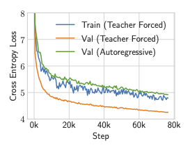
ST-Transformer training curves.
The blue curve corresponds to the training loss under teacher-forced training. While the teacher-forced validation loss is optimistic—since it conditions on ground-truth inputs—it can be interpreted as a lower bound on the achievable loss, representing the performance of an idealized autoregressive model with perfect inference.
To reduce the gap between teacher-forced and autoregressive performance, we experimented with scheduled sampling. However, this did not lead to meaningful improvements.
Conclusion
In summary, we demonstrated how a spatio-temporal transformer world model can be trained on the 1X World Model tokenized dataset in under 17 hours. We found that greedy autoregressive inference offered a practical balance of speed and accuracy. Despite its simplicity, the model achieved substantially lower loss values than other leaderboard entries and positioned 1st in the 1X World Model Compression Challenge.