This work implements and compares a variety of approximate inference techniques for the tasks of image de-noising (restoration) and image segmentation. In particular it provides implementations of Iterative Conditional Modes (ICM) a simple coordinate-wise gradient approach, Gibbs Sampling in an Ising model, a straight forward Markov Chain Monte Carlo method and Mean Field Variational Bayes in an Ising Model.
In machine learning inference is the task of combining our assumptions with the observed data. More specifically, if we have a set of observed data $\mathbf{Y}$, parameterized by a variable $\theta,$ then we wish to obtain the posterior,
\begin{equation} p(\mathbf{\theta} \mid \mathbf{Y}) = \frac{p(\mathbf{Y} \mid \mathbf{\theta}) p(\mathbf{\theta})}{p(\mathbf{Y})}. \end{equation}
The denominator is known as the marginal likelihood (or evidence) and represents the probability of the observed data when all of the assumptions have been propagated through and integrated out,
\begin{equation} p(\mathbf{Y}) = \int p(\mathbf{Y}, \mathbf{\theta}) d\theta. \end{equation}
Sometimes this integral is intractable (computationally or analytically) so we cannot exploit conjugacy to avoid its calculation. For this reason we have to make approximations to this integral.
Image Restoration
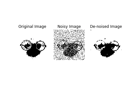
This can be demonstrated through image restoration, the process of cleaning up images that have been corrupted by noise. Image restoration of binary images.
The Model
Our task here is to build a model of images, in specific of binary or black-and-white images. Images are normally represented as a grid of pixels $y_i$ however the images we observe are noisy and rather will be a realisation of an underlying latent pixel representation $x_i$. Lets say that white is encoded by $x_i = 1$ and black with $x_i = −1$ and that the grey-scale values that we observed $y_i \in (0, 1)$. Our likelihood takes the form,
\begin{equation} p(\mathbf{y} \mid \mathbf{x}) = \frac{1}{Z_1} \prod_{i=1}^N e^{L_i(x_i)} \end{equation}
where $L_i(x_i)$ is a function which generates a large value if $x_i$ is likely to have generated $y_i$ and $Z_1$ is a factor that ensures that $p(\mathbf{y} \mid \mathbf{x})$ is a distribution. We have further assumed that the pixels in the image are conditionally independent given the latent variables x.